Making an AI: Part 3

If you have no idea what this is about yet, go to Making an AI: Part 2.

As a recap, last time I got the forward step working. This post, I got the learning part of the AI working.

Idea Explanation:

In our neural network, each layer, the weights, and the biases all affect the next layer. We want to tweak these, so that our final loss gets smaller. Moreover, we want to tweak these in the most efficient way possible: in other words, we want to have the most improvement in loss for a unit change in our weights or biases, and some of you may recognize this as trying to minimize the derivative of the loss.

Let’s focus on one node in our current layer, say this has a value of \(v_{l,i}\), where \(i\) represents the layer of our node, and \(j\) represents that this is the \(j\)th node in the layer \(i\). The value of \(v_{l,i}\) depends on the value of all of the nodes in the previous layer, but to make this simpler, let’s focus on only one node in the previous layer as well. Say the value of this node is \(v_{l-1,j}\). We know that

\[v_{l,i} = a(\sum_n (v_{l-1,n} w_{l,n,i}) + b_{l,i})\]

where \(w_{l,j,i}\) means this is the weight to multiply by the \(j\)th node to add to the value for the \(i\)th node of layer \(l\), \(b_{l,i}\) is the bias to add to the \(i\)th node of layer \(l\), and \(a()\) is the activation function.

To make this simpler, let’s focus on \(v_{l-1, j}\) and the weight related to it (\(w_{l,j,i}\)).

To go further in calculating the derivative, we need the chain rule. The chain rule states that if you have two functions (say \(f\) and \(g\)), the derivative of \(f(g(x))\) relative to \(x\) is \(f'(g(x))*g'(x)\). This is kind of intuitive: if \(f(x)\) is the brightness of a LED at a wattage \(x\), and \(g(t)\) is the wattage as a function of time, the change in brightness of the LED should be how quickly the LED’s brightness is changing at that wattage, multiplied by how quickly that wattage is changing.

Now, we can find the derivative of \(v_{l,i}\) relative to whatever we want.

If we want to find the derivative of \(v_{l,i}\) relative to \(w_{l,j,i}\), or how much we want to change \(w_{l,j,i}\), we can assume everything to be constant other than \(w_{l,j,i}\). Then, we can use the chain rule: the derivative of \(v_{l,i}\) is the derivative of \(a()\) evaluated at \(\sum_n (v_{l-1,n} w_{l,n,i}) + ... + b_{l,i}\) times the derivative of \(\sum_n (v_{l-1,n} w_{l,n,i}) + b_{l,i}\), which because everything is constant other than \(w_{l,j,i}\), is just \(v_{l-1,j}\). We also need to multiply by the how much we want to change \(v_{l,i}\) , so the derivative of \(w_{l,j,i}\) is

\[v_{l,i}'a'(\sum_n (v_{l-1,n} w_{l,n,i}))v_{l-1,j}\]

The derivative of the bias \(b_{l,i}\) is the derivative of \(a()\) evaluated at \(\sum_n (v_{l-1,n} w_{l,n,i}) + b_{l,i}\), multiplied by the derivative of that, which is just 1. This is then

\[v_{l,i}'a'(\sum_n (v_{l-1,n} w_{l,n,i}) + b_{l,i})\]

Finally, we need the derivative of \(v_{l-1,j}\), so that we can use it to adjust the weights of layer \(l-1\). This is pretty similar to the derivative of the weight: \(v_{l,i}'a'(\sum_n (v_{l-1,n} w_{l,n,i}) + b_{l,i})v_{l,i,j}\)

This process of calculating the derivative can be done for every pair of nodes between layer \(l\) and \(l-1\). Then, we can just do this for every layer. Because we need the derivative of our current layer’s nodes, which comes from the layer after this current layer, we have to start from the end and adjust stuff going backwards. This is where the word “backpropogation” comes from: you propogate the derivative back layer by layer.

Now, you can do this a bunch of times, and tweak everything a little bit, and hopefully it’ll learn to the data that you give it.

Code Explanation:

My code is here: github.com

As a recommendation from my dad, I commented everything a lot, and just gave the link here.

Note: some code from the last post may have changed.

Results

I decided to try to make an xor gate instead of a color detector because discriminating between yellow and purple can be done with a line (or techincally a plane, but same idea) but you can’t do a linear fit on an xor gate. If you put the outputs of an xor gate on a graph, you get this:

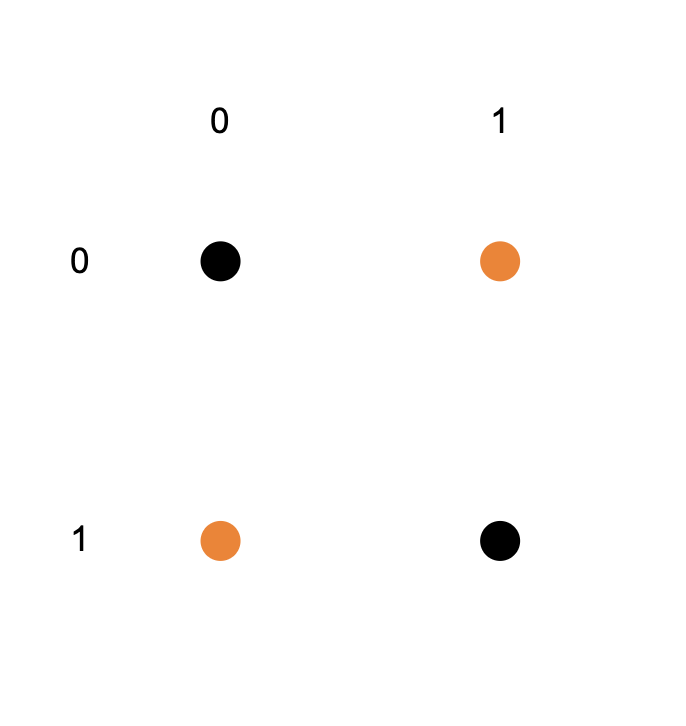
where the numbers on the top are what you input into the xor as the first number and the numbers on the side are what you input into the xor as the second number, and the dots are what the xor is returning (black = 0, orange = 1).

You can try to separate this image into two parts with a single line, where one side only has orange dots, and the other side only has black dots, but you’ll probably quickly find out that it isn’t possible. This is what makes this harder than the color separation: If you put the colors on a graph, you can find a line that splits yellow and purple.

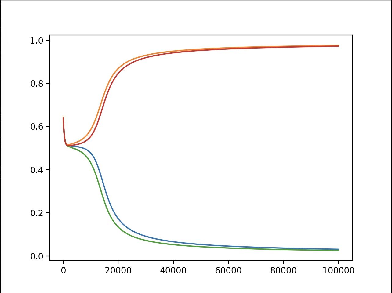
Anyway, here are what values the model returned, plotted by generations (or maybe epochs?):

Test 1:

Test 2:

Test 3:

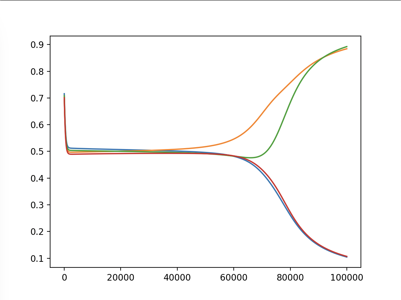
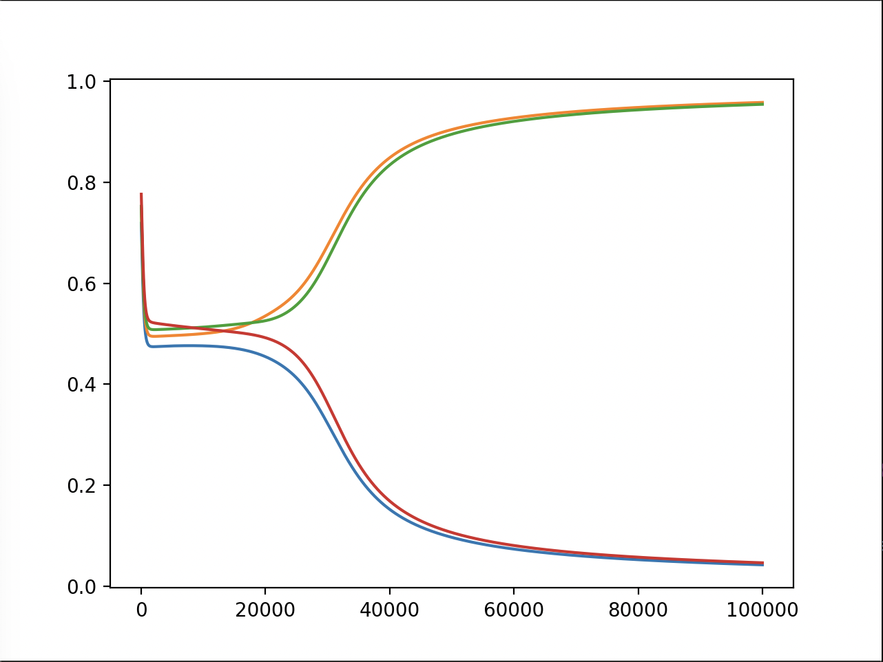
As we can see in all of the tests, the model does very well, putting two of the values in the 1 and two of the values in the 0 (we don’t know which two, but I’ll show that it actually did it right later). At the start, the outputs are random, and we can see a clear centering to 0.5, probably because that minimizes the loss if you can only use lines to split the plane. But then, in all of the tests, eventually the outputs form two groups that go to 1 and 0.

In test 3, it took much longer for the two groups to start to diverge. This is because I tried to make the model smaller to see if it would still learn and converge, which it did.

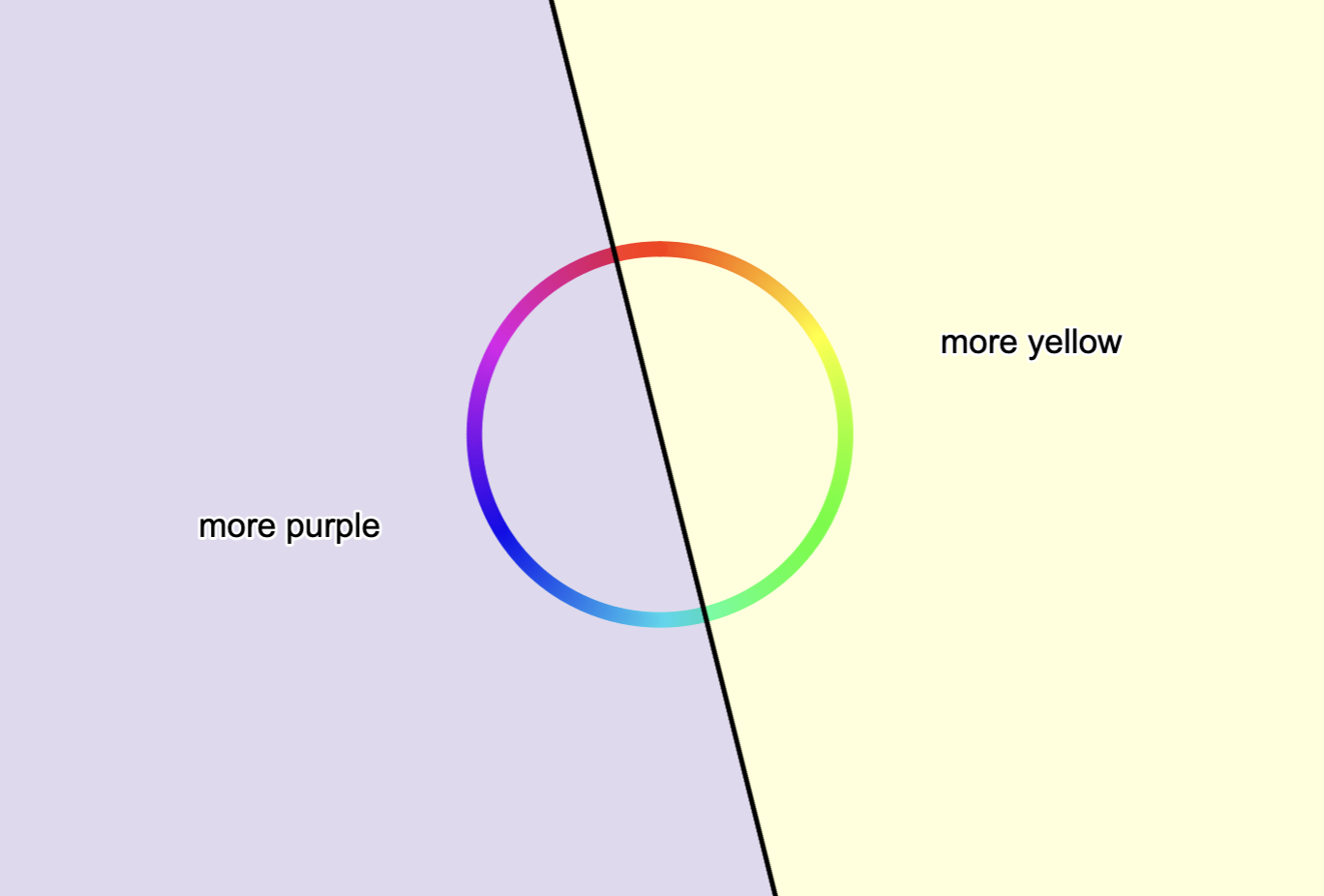
Another possible way to visualize this is to ask the ai for the answer to those dots and graph them, just with … a lot more.

Test 4:

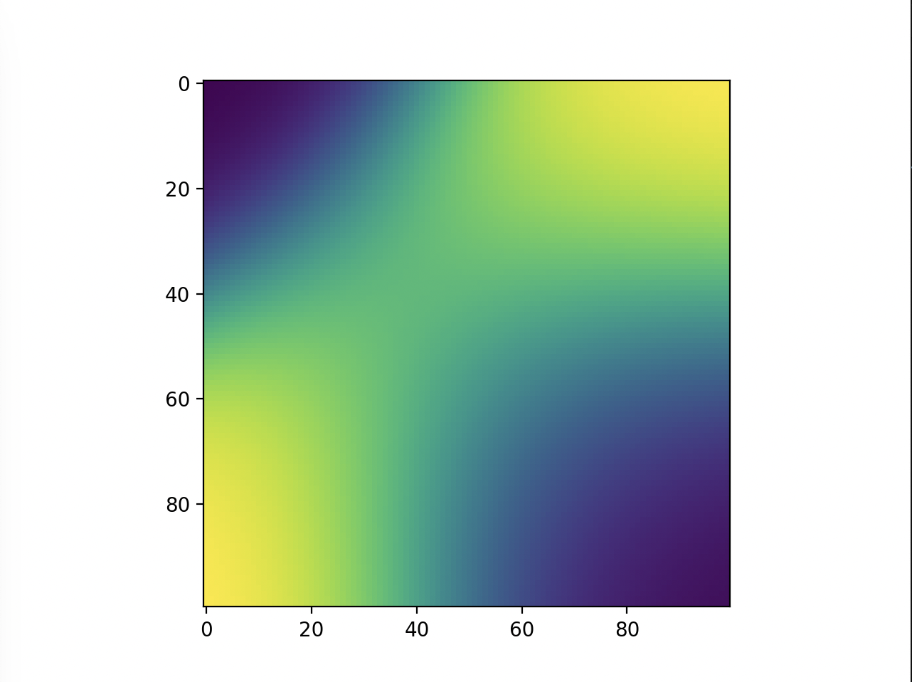
Test 5:

Here, more purple means closer to 0 and more yellow means closer to 1. Now, we can see that the model does in fact do the xor, and more on how it does it. Instead of differentiating by a line, it makes a band of yellow going from the bottom left to the top right or a band of purple going from the top left to the bottom right.

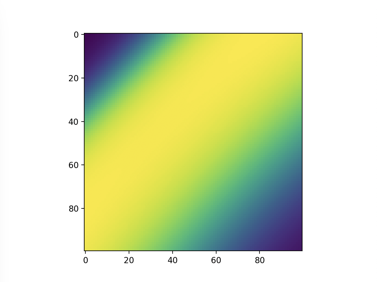
Then, I thought it would be cool to see how the model learned over time, so I made a gif of this same graph throughout the generations (epochs?).

Test 6:

Test 7:

We can see here many of the things we observed in the original graphs: the reset of everything to 0.5 at the start, then the slow divergence.

Conclusion

Although this is a rudimentary network, this still proves the concept of an AI learning. The purpose was also to show people that the most basic AI’s aren’t as complicated as most people think, and to encourage people to try it themselves. Regardless, AI can get a lot more complicated, like with implicit layers, transformers, and so on.